Advanced scale bar and compass annotations

1. Setup

This vignette demonstrates how to use the advanced customization options available in annotation_scalebar() and annotation_compass() from the ggmapcn package.

We will use the standard North Carolina shapefile provided by the sf package as our base map.

library(ggplot2)
library(sf)
#> Linking to GEOS 3.11.2, GDAL 3.8.2, PROJ 9.3.1; sf_use_s2() is TRUE
library(ggmapcn)

# Load example data
nc <- sf::st_read(system.file("shape/nc.shp", package = "sf"), quiet = TRUE)

# Create a base map object
base_geo <- ggplot() +
  geom_sf(data = nc, fill = "grey90", color = "grey40") +
  theme_minimal()

base_geo

2. Scale bars in a projected CRS

Scale bars are most accurate when used with a projected Coordinate Reference System (CRS). Here, we project the map to EPSG:32617 (UTM Zone 17N).

You can control the position using location (e.g., "bl" for bottom-left, "tr" for top-right) and adjust the relative width using width_hint.

base_proj <- base_geo +
  coord_sf(crs = 32617) +
  theme(axis.title = element_blank())

# Default scale bar at bottom-left
base_proj +
  annotation_scalebar(location = "bl")

# Top-right scale bar with custom width hint
base_proj +
  annotation_scalebar(
    location   = "tr",
    width_hint = 0.5
  )

3. Scale bar styles

annotation_scalebar() supports multiple styles: "segment", "ticks", and "bar". You can also customize colors and text visibility.

# 1. Segment style
p_segment <- base_proj +
  annotation_scalebar(
    location = "bl",
    style    = "segment",
    label_show = "all"
  )
p_segment

# 2. Ticks style
p_ticks <- base_proj +
  annotation_scalebar(
    location = "br",
    style    = "ticks"
  )
p_ticks

# 3. Bar style with custom colors
p_bar <- base_proj +
  annotation_scalebar(
    location = "tl",
    style    = "bar",
    bar_cols = c("black", "white")
  )
p_bar

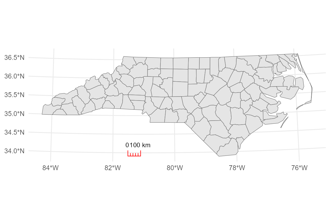
You can also set a fixed distance width (e.g., 100km) and change the line colors:

base_proj +
  annotation_scalebar(
    location     = "bl",
    fixed_width  = 100000,   # 100 km in meters
    display_unit = "km",
    line_col     = "red"
  )

4. Geographic CRS: Approx distance vs. Degrees

When plotting unprojected data (Latitude/Longitude, EPSG:4326), accurate distance calculation is difficult.

• geographic_mode = "approx_m": Attempts to calculate distances in meters (approximation).
• geographic_mode = "degrees": Shows the scale in decimal degrees.

# Approximate meters
base_geo +
  coord_sf(crs = 4326) +
  annotation_scalebar(
    location        = "bl",
    geographic_mode = "approx_m"
  )
#> Warning: Scale bar is approximate in geographic CRS (degrees). Distances vary
#> with latitude. For accuracy, use a projected CRS, or set `geographic_mode =
#> "degrees"`.

# Degrees
base_geo +
  coord_sf(crs = 4326) +
  annotation_scalebar(
    location        = "bl",
    geographic_mode = "degrees"
  )

5. Basic compass (Grid North)

Add a north arrow using annotation_compass(). You can adjust the size and padding using grid::unit().

# Default classic arrow
base_geo +
  annotation_compass(
    location = "tl",
    style    = north_arrow_classic()
  )

# Custom size and padding
base_geo +
  annotation_compass(
    location = "tl",
    height   = grid::unit(0.8, "cm"),
    width    = grid::unit(0.8, "cm"),
    pad_x    = grid::unit(0.3, "cm"),
    pad_y    = grid::unit(0.3, "cm")
  )

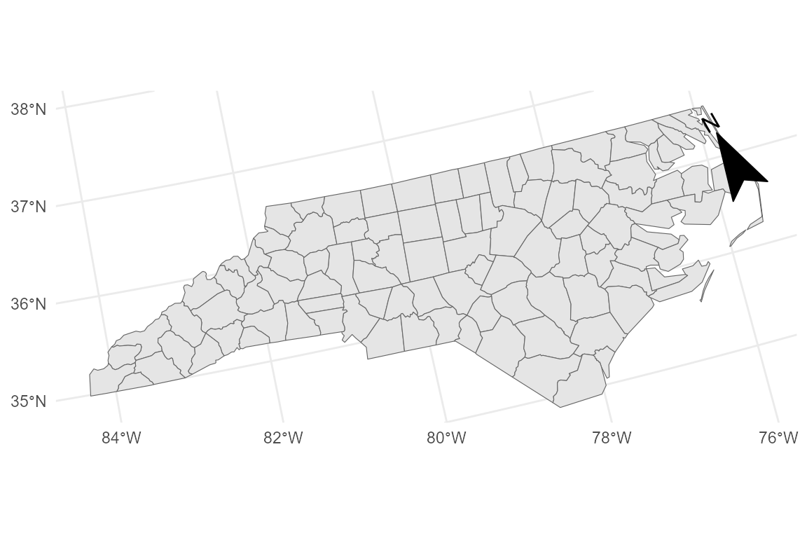
6. True North vs. Grid North

In many projections (like Lambert Conformal Conic), “Grid North” (straight up on the page) is different from “True North” (the direction to the North Pole).

Use which_north = "true" to automatically calculate the convergence angle and rotate the compass.

# Define a Lambert Conformal Conic projection
base_lcc <- base_geo +
  coord_sf(crs = "+proj=lcc +lon_0=-100 +lat_1=33 +lat_2=45") +
  theme(axis.title = element_blank())

# True North (automatically rotated)
base_lcc +
  annotation_compass(
    which_north = "true",
    location    = "br",
    style       = compass_rose_simple()
  )

# Grid North with manual rotation
base_lcc +
  annotation_compass(
    which_north = "grid",
    rotation    = 30,
    location    = "tr",
    style       = north_arrow_solid()
  )

7. Compass styles

ggmapcn provides various styles, including the unique compass_sinan() (referencing the ancient Chinese compass).

p_classic <- base_proj +
  annotation_compass(
    location = "tl",
    style    = north_arrow_classic()
  )

p_rose <- base_proj +
  annotation_compass(
    location = "br",
    style    = compass_rose_classic()
  )

p_sinan <- base_proj +
  annotation_compass(
    location = "tl",
    style    = compass_sinan()
  )

p_classic

p_rose

p_sinan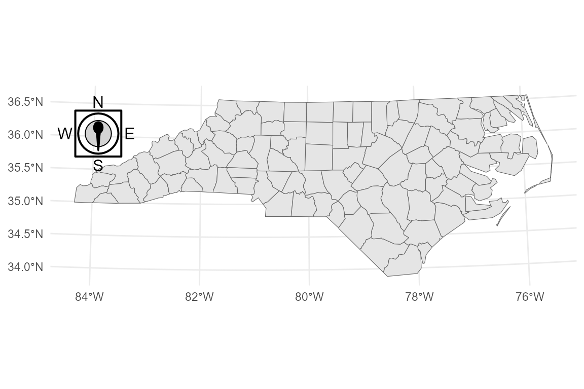

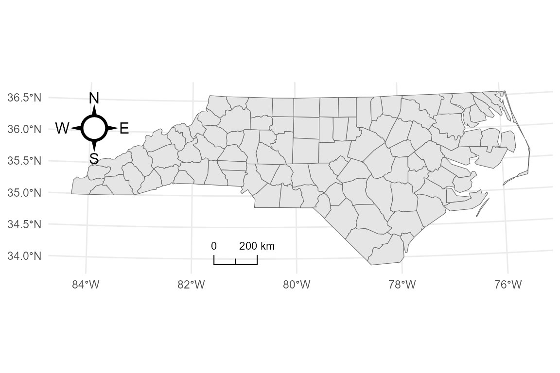
8. Combining scale bar and compass

Finally, you can layer both annotations onto a single map.

base_proj +
  annotation_scalebar(
    location   = "bl",
    style      = "ticks",
    width_hint = 0.3
  ) +
  annotation_compass(
    location = "tl",
    style    = compass_rose_circle()
  )